Sheet 4
††course: Optimization in Machine Learning††semester: FSS 2023††tutorialDate: 27.04.2023††dueDate: 12:00 in the exercise on Thursday 27.04.2023While there are \totalpoints in total, you may consider all points above the standard to be bonus points.
Exercise 1 (Lower Bounds).
In this exercise, we will bound the convergence rates of algorithms which pick their iterates from
We consider the function
-
(i)
To understand our function better, we want to view it as a potential on a graph. For this consider the undirected graph with vertices
and edges
Draw a picture of this graph.
Solution.
The graph is simply a chain
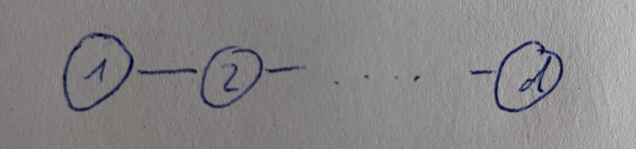
∎
-
(ii)
We now interpret as a quantity (e.g. of heat) at vertex of our graph . Our potential decreases, if the quantities at connected vertices and are of similar size. I.e. if is small. Additionally there is a pull for to be equal to . Use this intuition to find the minimizer of .
Solution.
The minimizer is since and . ∎
-
(iii)
The matrix with
is called the “Graph-Laplacian” of . The degree of vertex are the number of connecting edges. Calculate for and prove that
Solution.
The Graph-Laplacian of is given by
Let then
similarly looking at the cases individually immediately reveals
-
(iv)
Prove that the Hessian is constant and positive definite to show that is convex. Prove that the operator norm of is smaller than . Argue that
is therefore -smooth.
Solution.
Taking the derivative of the gradient we calculated previously yields
To show positive definiteness, let be arbitrary
To find the largest eigenvalue of we want to calculate the operator norm. For this we use to get
Thus we get
Since the operator norm coincides with the largest absolute eigenvalue for symmetric matrices, this proves our claim. Finally -smoothness of follows from
-
(v)
Assume and and that is chosen with the restriction
To make notation easier we are going to identify with an isomorph subset of sequences
then is a subset of for . Prove inductively that
Solution.
We have the induction start by
Now assume
then by our selection process . But then
We therefore have .
Notice how the low connectedness of the graph limits the spread of our quantity . A higher connectedness would allow for information to travel much quicker. ∎
-
(vi)
We now want to bound the convergence speed of to . For this we select .
Note: We may choose a larger dimension by defining on the subset in . The important requirement is therefore . But without loss of generality we assume equality.
Use the knowledge we have collected so far to argue
Solution.
Since we know that
-
(vii)
To prevent the convergence of the loss to we need a more sophisticated argument. For this consider
Argue that on the functions and are identical. Use this observation to prove
Solution.
Let . Then using we have
using for all for the second equality sign. Since we therefore can replace with at will to get
-
(viii)
Our goal is now to calculate . Prove convexity of and prove that
is its minimum. Then plug our solution into (or , since is in the subset after all), to obtain the lower bound
Solution.
We have
where is the Graph-Laplacian for . Then the Hessian is obviously positive definite
as we could apply the same arguments as for . So is convex. We now plug into to verify the first order condition, proving it is a minimum
We now know that
using again. ∎
-
(ix)
Argue that we only needed
with upper triangular matrices to make these bounds work. Since adaptive methods (like Adam) use diagonal matrices , they are therefore covered by these bounds.
Solution.
We only needed which we proved by induction using only this fact about . Since upper triangular matrices do not change this fact, we may as well allow them. ∎
-
(x)
Bask in our glory! For we have proven that …? Summarize our results into a theorem.
Solution.
Theorem (Nesterov).
Assume there exists upper triangular matrices such that the sequence in is selected by the rule
for a convex, -smooth to minimize. Then up to there exists a convex, -smooth function such that
for .
∎
-
(xi)
(Bonus) If you wish, you may want to try and repeat those steps for
to prove an equivalent result for -strongly convex functions. Unfortunately finding is much more difficult in this case. Letting makes this problem tractable again with solution
Exercise 2 (Conjugate Gradient Descent).
Consider a quadratic function
for some symmetric and positive definite and consider the hilbert space with
-
(i)
Prove that is a well-defined scalar product. Convince yourself that
Solution.
Bilinearity is trivial, the positive-definiteness follows from this property of . We have
-
(ii)
Determine the derivative of in
Hint.
Recall that is the unique vector satisfying
Solution.
We need
= lim_v→0 —f(x+v) - f(x) - ⟨∇ H f(x) , v⟩ H — ∥v∥ H We can bound the fraction of norms by a constant from below due to equivalence of all norms in . This lower bound on the second fraction forces the first fraction to converge to zero. But this implies that
by the definition (and uniqueness) of . Thus the gradient we are looking for is
-
(iii)
Since gradient descent in the space is therefore computationally the Newton method, we want to find a different method of optimization. Consider an arbitrary set of conjugate (-orthogonal) directions , i.e. , and for some starting point the following descent algorithm:
Optimizing over in this manner is known as “line-search”. Using prove that
Deduce that conjugate descent (CD) converges in steps.
Solution.
We proceed by induction. The induction start with is obvious. Let us now consider . By its definition we have
the minimizer is therefore . This removes the component leaving us with the components and up. Note that for all by induction. Similarly we can see that this is a minimum in the span of , as we have removed those components completely and
Since we can not touch the other components due to -orthogonality, this is the best we can do. ∎
-
(iv)
If we had , then this algorithm would be optimal in the set of algorithms we considered in the previous exercise. Unfortunately the gradients are generally not conjugate. So while we may select an arbitrary set of conjugate , we cannot select the gradients directly.
Instead we are going to do the next best thing and inductively select such that
using the Gram-Schmidt procedure to make conjugate to . Since Gram-Schmidt is still computationally too expensive for our tastes, you please inductively prove
assuming is -dimensional. I.e. is a “-Krylov subspace”.
Solution.
The induction start follows directly from
and the definition of . Assume we have the claim for , then
As by the induction hypothesis, we therefore have
Since they are by the induction hypothesis also in the span
Since the space on the left is dimensional, we have equality. ∎
-
(v)
Argue that is orthogonal to every vector in and inductively deduce either
which implies , or has full rank. Deduce from the -Krylov-subspace property, that is already -orthogonal to .
Hint.
.
Solution.
By the selection process of , we have
assume were not orthogonal to . Then there would exist such that
By the Taylor approximation we therefore have
so there exists a small such that . But this is a contradiction since was optimal.
is therefore orthogonal to . So if it is not zero, has (as the span of both) full rank. being orthogonal to also implies it is orthogonal to , since that is a subspace of by the Krylov property. But this implies is -orthogonal to . ∎
-
(vi)
Collect the ideas we have gathered to prove the recursively defined
are -conjugate and have the same span as the gradients up to .
Solution.
These are the same we would obtain using Gram-Schmidt on the gradients. In fact this is Gram-Schmidt together with the fact that is already -orthogonal to the . So only the last summand remains. ∎
-
(vii)
To make our procedure truly computable, we want to show
Hint.
Proving
should allow you to conclude Then it makes sense to calculate
by solving its optimization problem. Finally you may want to consider and .
Solution.
We have
This implies and therefore
where we have used , which follows from and .
Now we need to find . But the first order condition
= d dα f(x_k-1 - αv_k) implies
Before we put things together, note that by definition of
since is orthogonal to . From this we get
So we finally get
-
(viii)
Summarize everything into a pseudo-algorithm for conjugate gradient descent (CGD) and compare it to heavy-ball momentum with
using identical as CGD.
Solution.
We set or later
determine the step-size
and finally make our step
Using the fact and inserting into the last equation, we notice
that CGD is identical to HBM with certain parameters , . ∎
Exercise 3 (Momentum).
In this exercise, we take a closer look at heavy-ball momentum
-
(a)
Find a continuous function such that
Prove that is -strongly convex with , -smooth with and has a minimum in zero.
Solution.
We define
note that it is continuous in and and therefore everywhere, and that it has the correct derivative. Further note that
is the derivative of in the following sense:
which follows from differentiability of on its segments with the fundamental theorem of calculus and continuity between segments. Thus we have
For the Bregman divergence this implies
thus is -strongly convex and -smooth. ∎
-
(b)
Recall, we required for convergence of HBM
Calculate the optimal and to minimize the rate .
Solution.
To minimize , we first set
and then proceed to minimize this over . Which results in
which is monotonously falling for
and monotonously increasing otherwise. Therefore its minimum is at equality. Thus
This results in
-
(c)
Prove, using heavy ball momentum on with the optimal parameters results in the recursion
Solution.
Using our previous results about optimal rates we have for
Thus
∎
-
(d)
We want to find a cycle of points , such that for we have
Assume , and and use the heavy-ball recursion to create linear equations for . Solve this linear equation. What does this mean for convergence?
Solution.
We have
Multiplying both sides by , using and and similarly and reordering, we get
solving this system of equations results in
As we have managed to find a cycle of points, HBM does not converge to the minimum at zero in this case. Note: it is also possible to show that this cycle is attractive if you start in an epsilon environment away from these points. ∎
-
(e)
Implement Heavy-Ball momentum, Nesterov’s momentum and CGD https://classroom.github.com/a/f3PnRxTs.
-
(a)